data

Micropaleontologic and Oceanographic Data

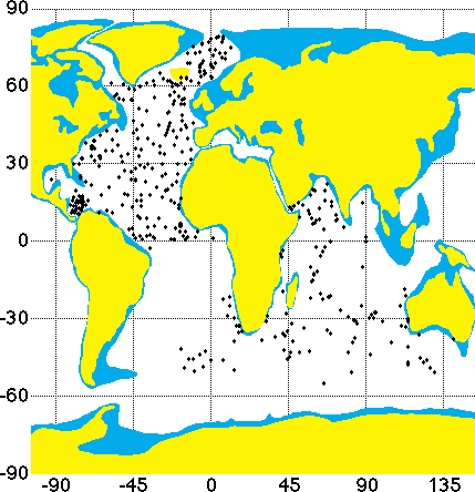
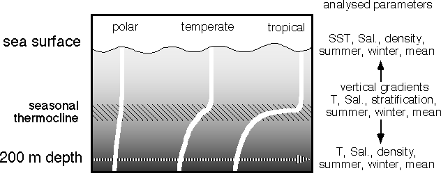
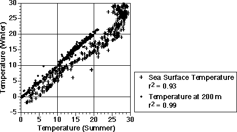
Figure 1 shows the core locations of the 461 Holocene Atlantic and Indian Ocean samples analysed by Bé and Hutson (1977), Hutson and Prell (1980), and Kipp (1976), whose data are used in this study. The average number of counted specimens of planktic foraminifera in these samples is 494 + 180 (standard deviation), with about 300 as a minimum, except in some highly dominated high latitude samples, and a record of 35 species and 6 variants from the size fraction >150 µm. Most species are rare in the assemblages. The number of counted specimens allows for statistically significant analyses of relative abundances greater than about 1 %. All lower relative abundance counts are subject of statistical uncertainty. The data is available from the National Geophysical Data Center (NGDC). According to Kipp (1976) the taxonomy follows Parker (1962, 1967), with modifications by Bé (1967) and Bé and Hamlin (1967). Saito et al. (1981) provided additional descriptions of species concepts used by CLIMAP project members (1976, 1981). Generic assignments in this paper follow Hemleben et al. (1989).

Summer and winter temperature, salinity, and water density at the sea surface and at 200 m depth were extracted for each core location from the Levitus (1982) database made available by the National Oceanographic and Atmospheric Administration (NOAA). From this data I computed the vertical temperature and salinity gradient between the sea surface and 200 m depth and of the water density as a measure of stratification, separately for summer and winter according to the Levitus (1982) definitions (see Fig. 2). Vertical gradients are expressed as "surface value minus value at 200 m depth". Seasonal variation (seasonality) is expressed as "summer value minus winter value". The depth of 200 m was chosen as a reference horizon below the seasonally variable mixed layer. Such a reference is necessary because some species descend below the seasonal thermocline during their ontogenetic cycle and may react to conditions below the mixed layer. The oceanographically more meaningful conditions at the base of the mixed layer present problems with the definition of the seasonal thermocline, the steep gradients at this level, and in some ocean areas a seasonal thermocline does not exist for part of the year. Figure 3 shows little seasonal change at 200 m depth on a global scale. Oceanographic conditions at that depth can be used to characterise gradients between the mixed layer and the central waters.

Biogeographic distribution maps of individual species have been published by Bé and Hutson (1977), and Kipp (1976). They will not be duplicated in this paper but will be applied in the interpretations. It is recommended to use these maps and references to other biogeographic work in these publications, with results presented here.

Figure 1: Locations of 461 core top samples analysed by CLIMAP (1976, 1981), Bé and Hutson (1977), and Kipp (1976) whose data is used in this paper. Geographic gaps in the data delineate areas of moderate to bad carbonate preservation from where samples have been excluded. Dark pattern marks shelf areas.

Figure 2: Physical parameters extracted from the Levitus (1982) database and computed from this data. The depth of 200 m lies beyond most seasonal variation in the physical marine environment below the seasonal thermocline (Fig. 3). White lines indicate vertical temperature variation (schematic) in the major ocean areas. Note the different shape and strength of the seasonal thermocline and subsequent problems to define reprodicible levels, which would have made comparisons between different ocean areas and different seasons difficult.

Figure 3: Correlation of summer and winter water temperatures at the sea surface and at 200 m depth based on oceanographic data extracted for each core location (Fig. 1) from the Levitus (1982) database. Note scatter in the correlation of sea surface temperatures and differences in the correlation between different segments of the data cloud. In the tropics a linear correlation hardly exists. Physical conditions at 200 m are nearly constant over the year and are used to characterise conditions below the seasonal thermocline.

back to table of contents
access to all figures and tables

Micropaleontologic and Oceanographic Data