Figures and Tables


This page gives acces to all figures and tables in the atlas on
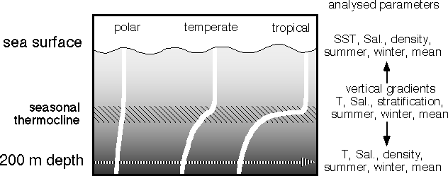
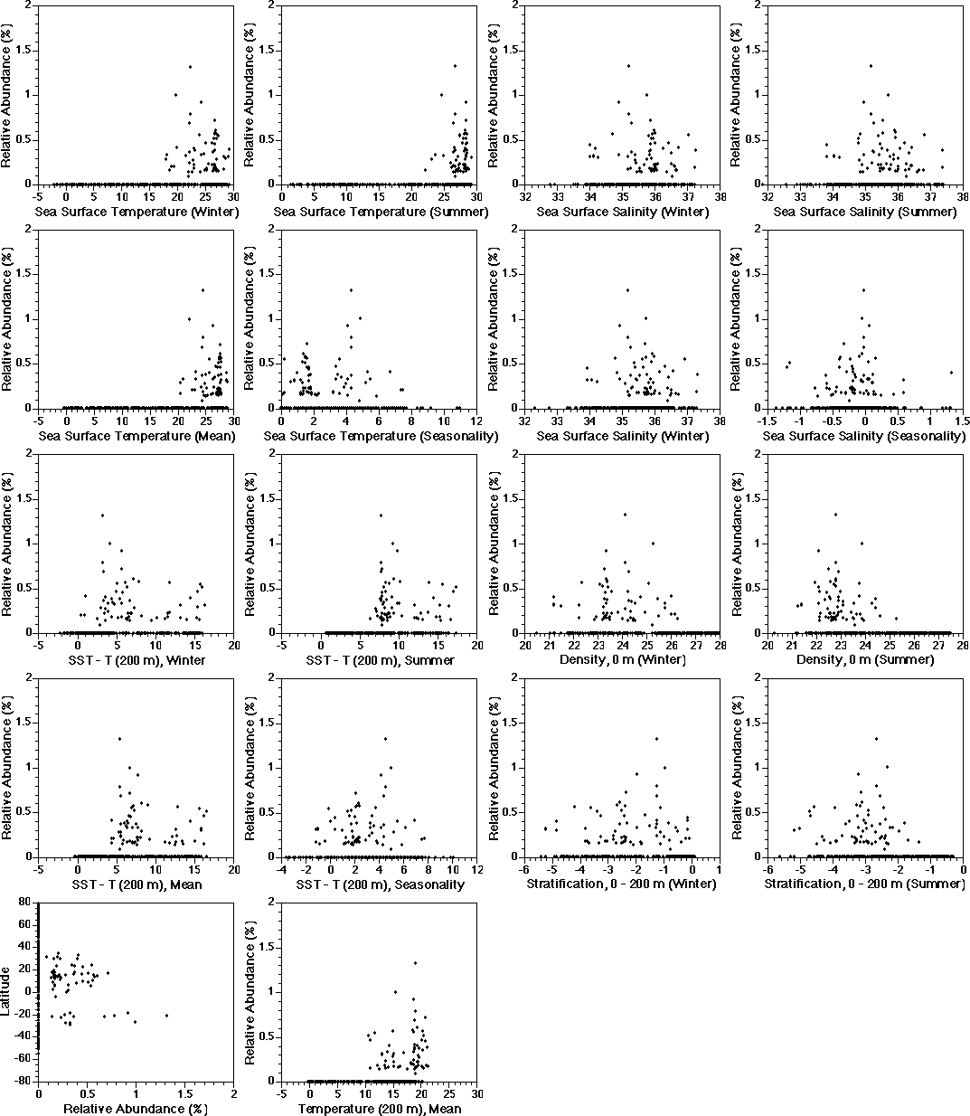
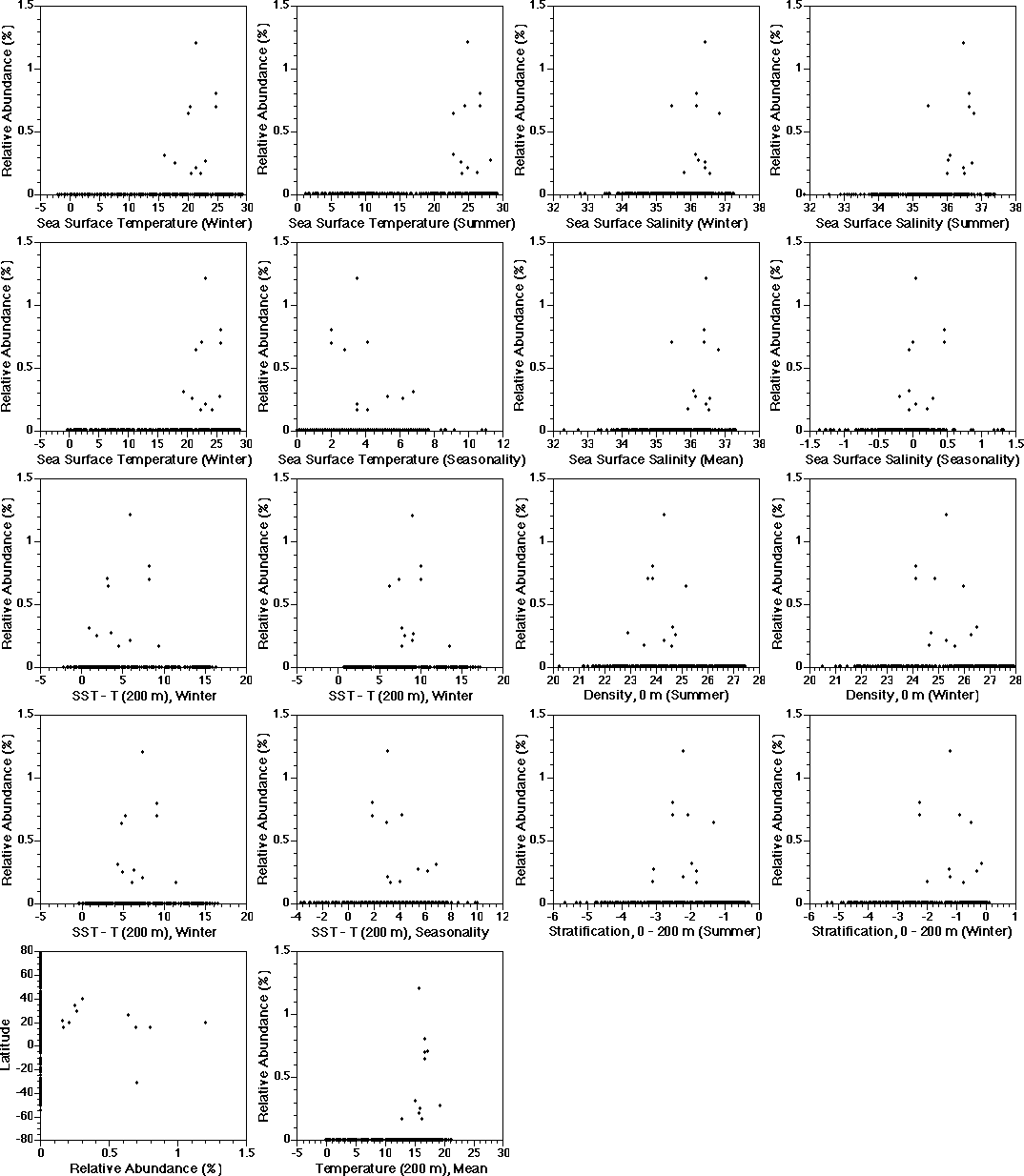
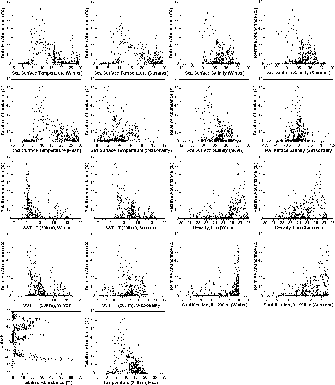
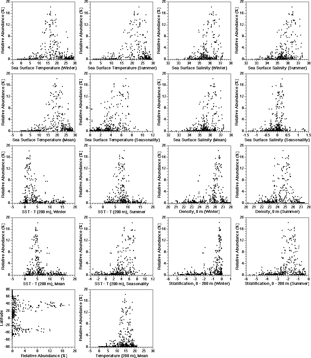
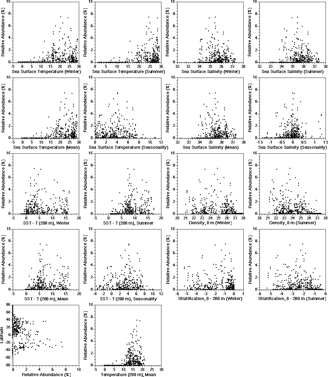
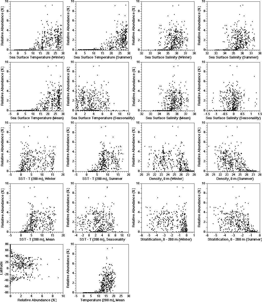
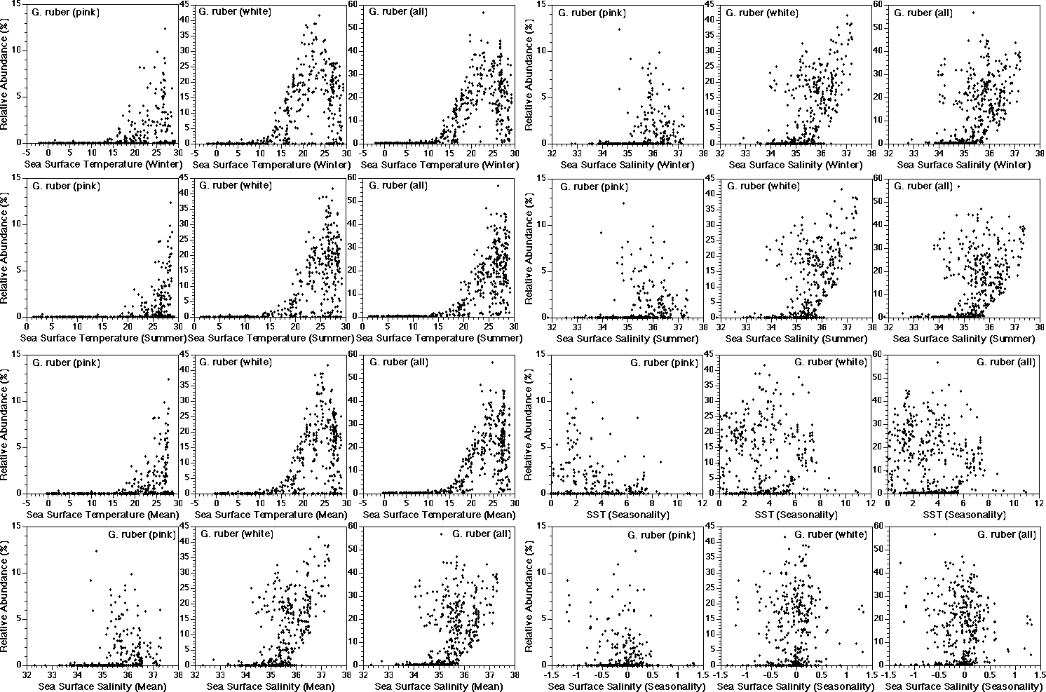
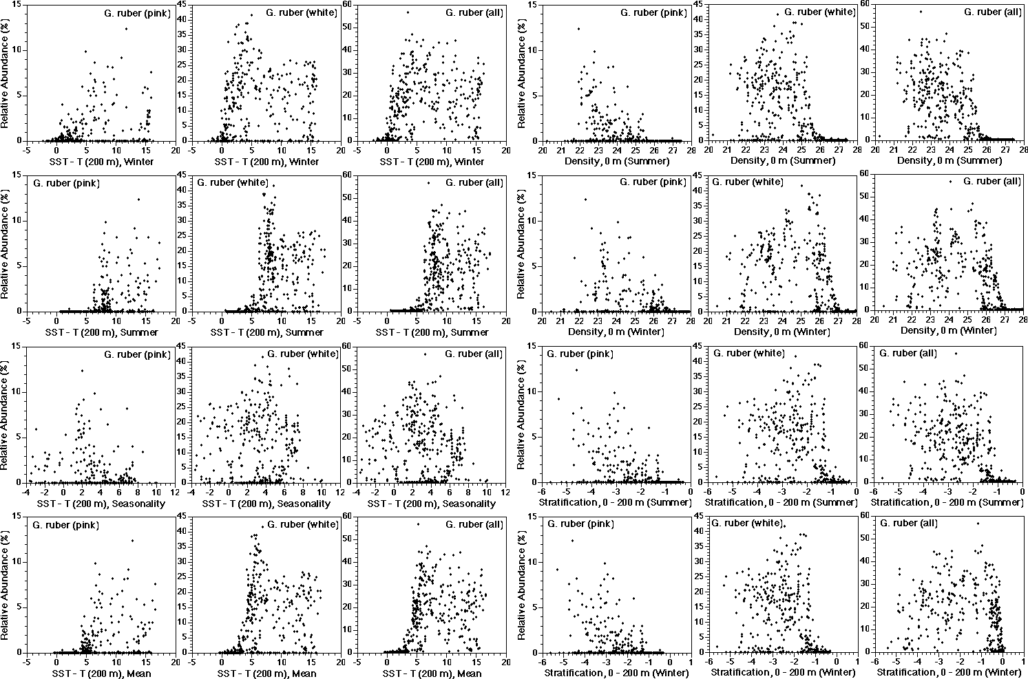
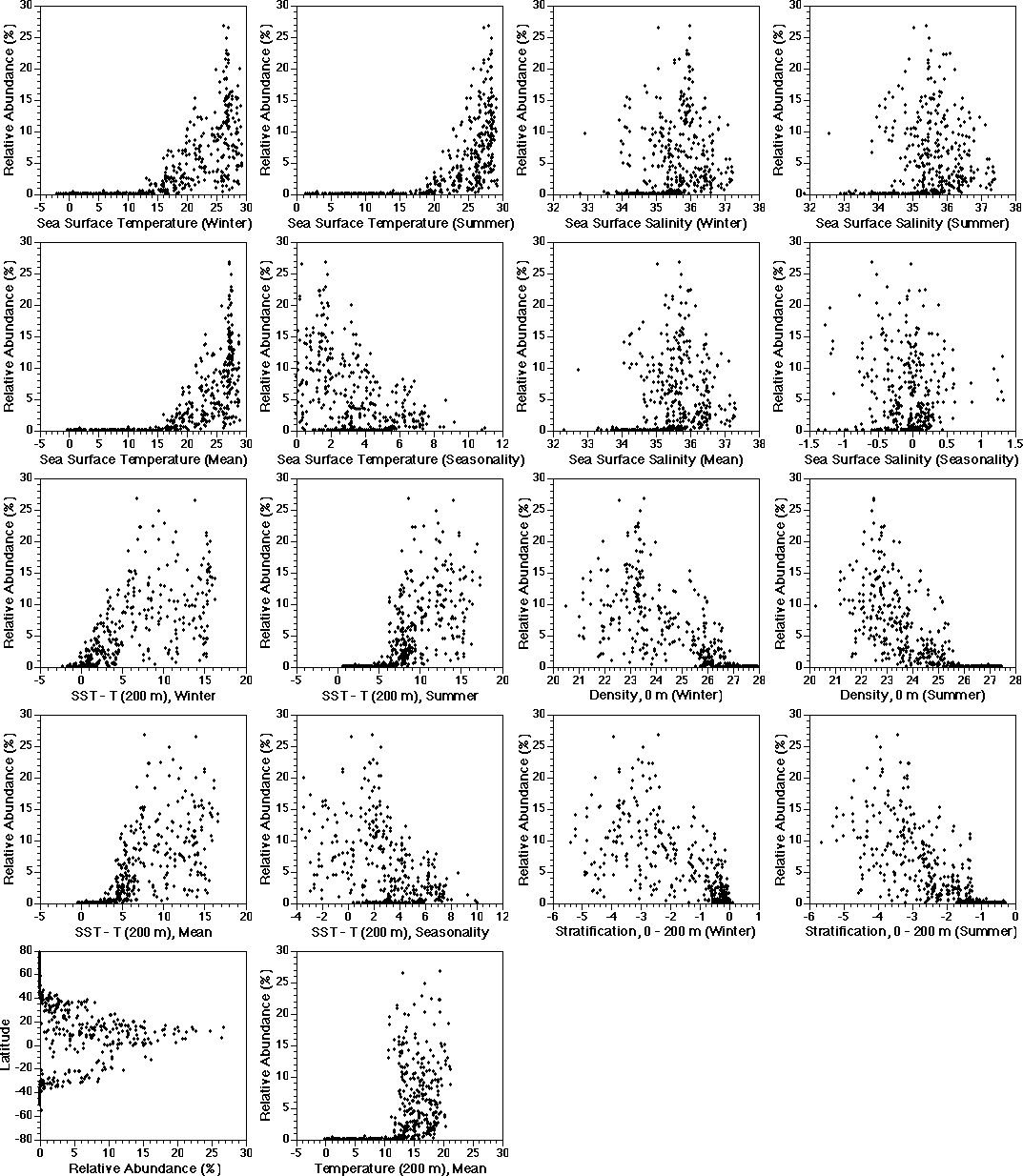
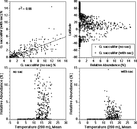
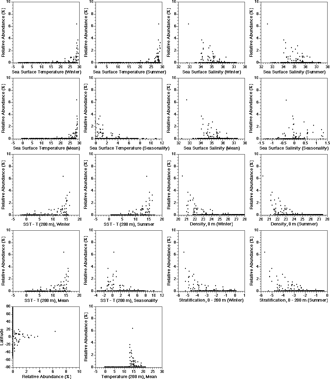
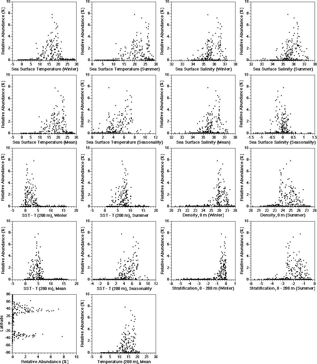
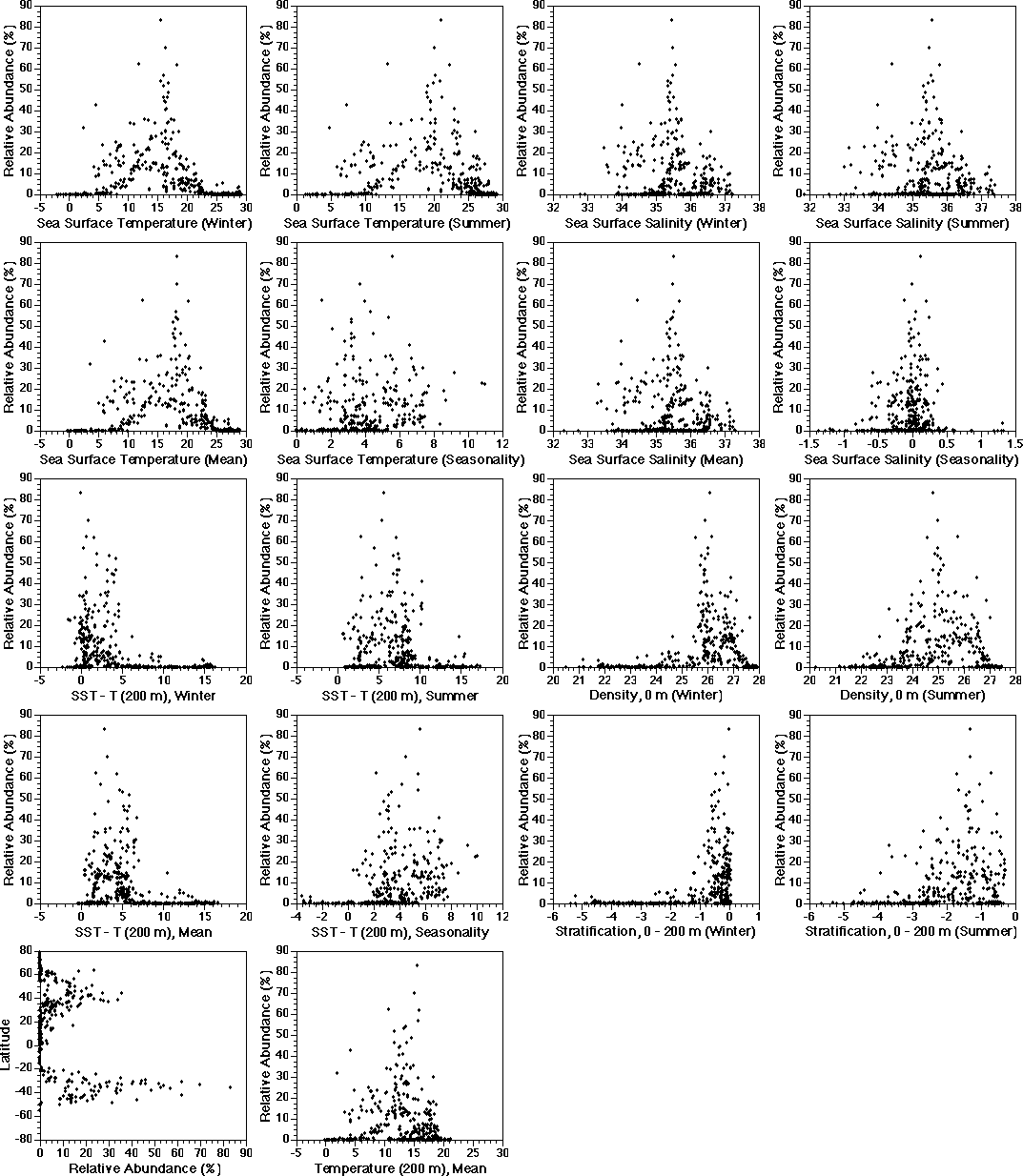
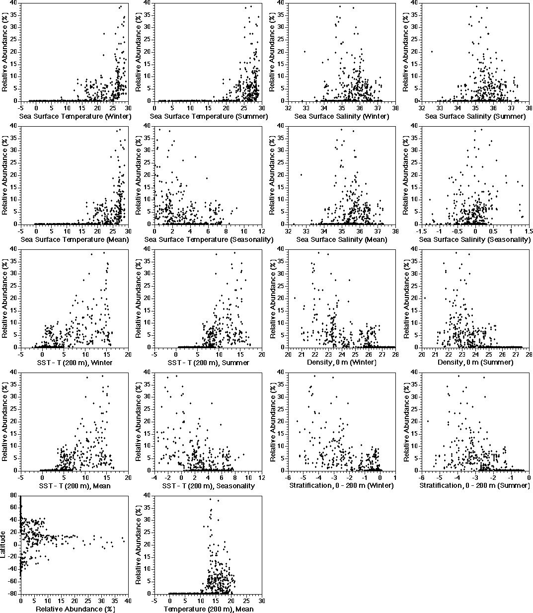
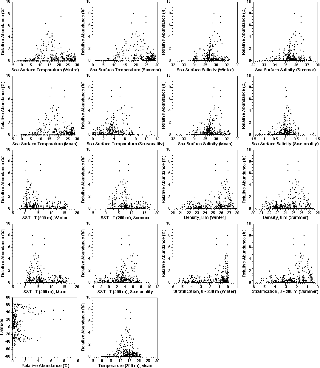
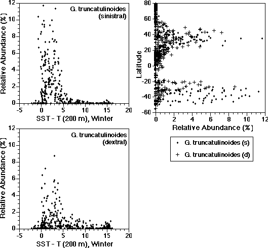
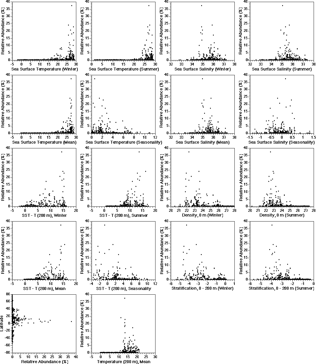
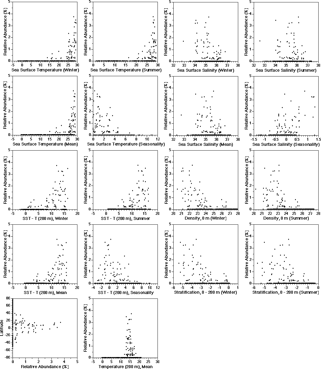
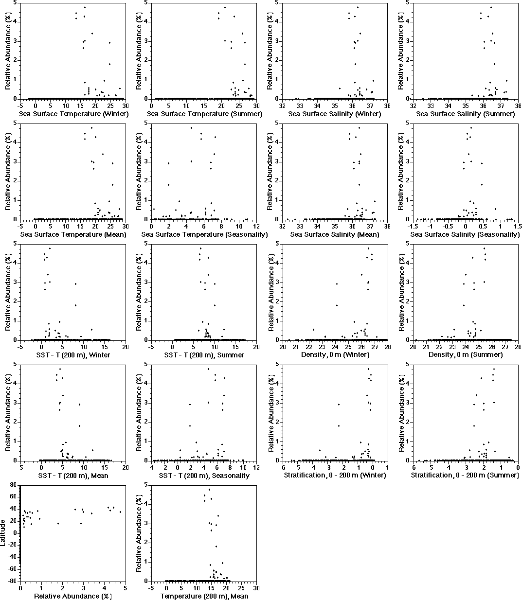
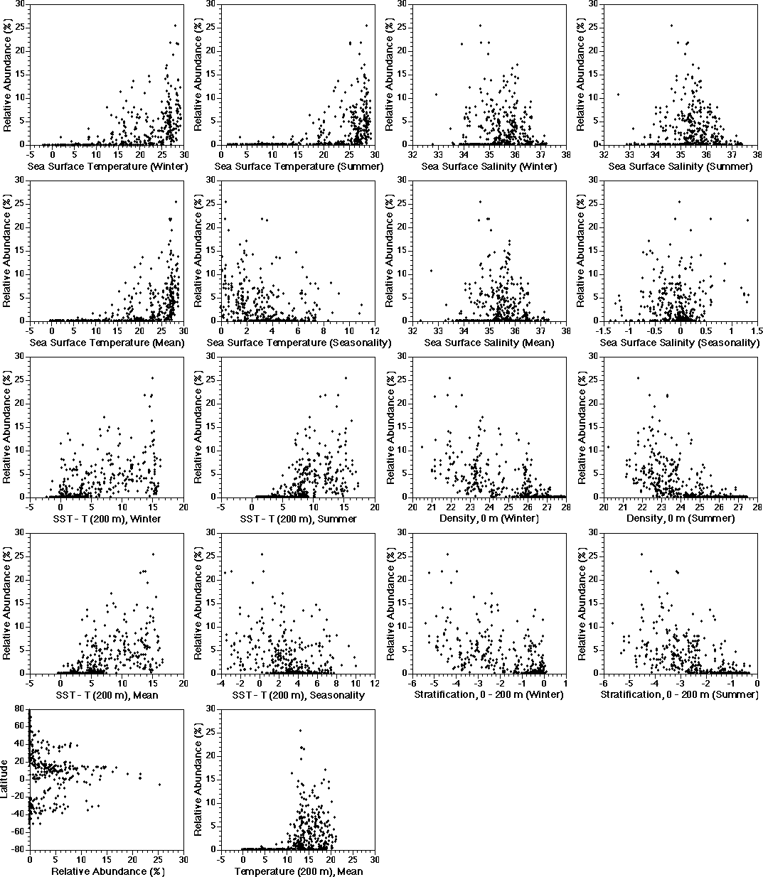
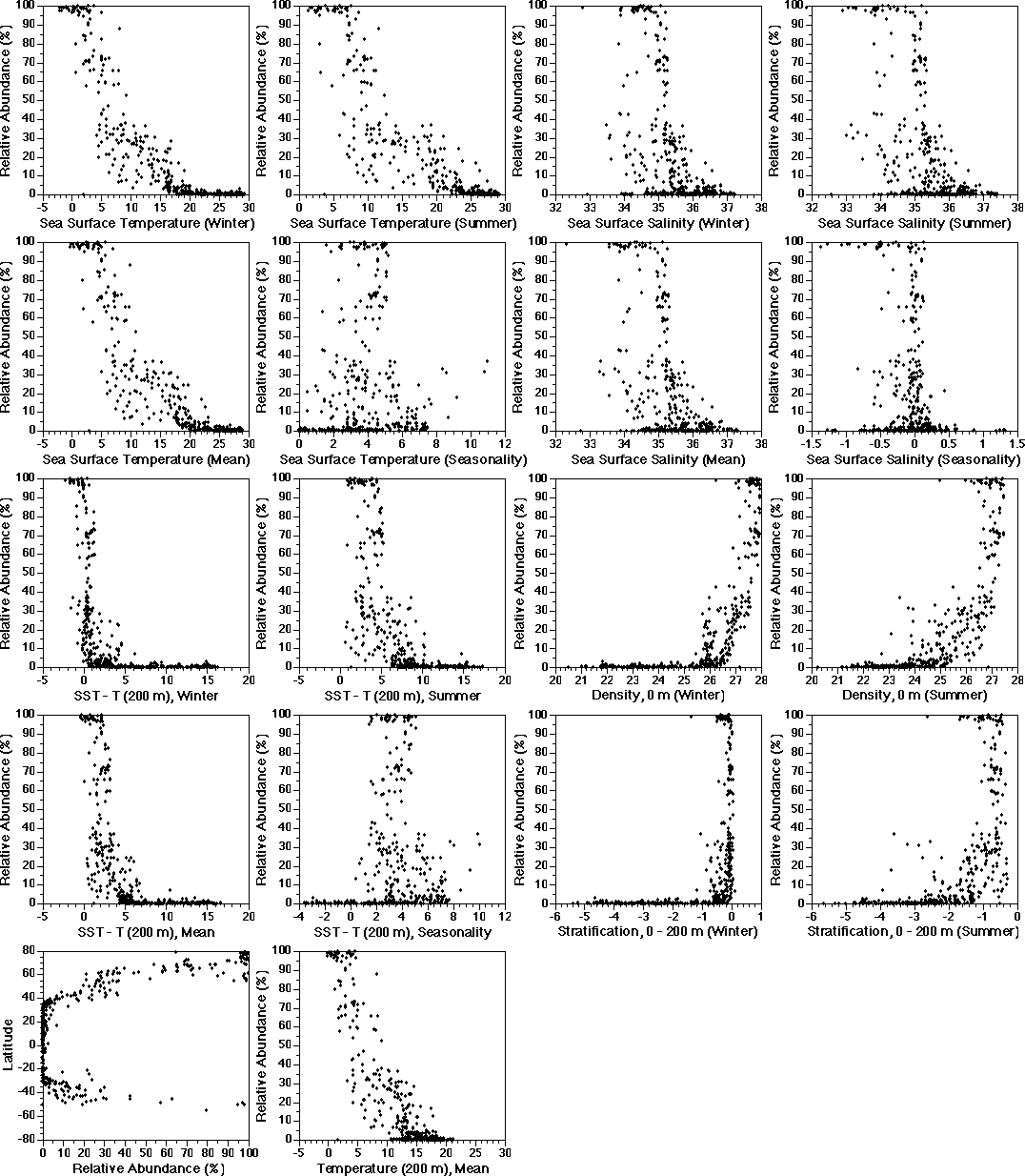
"Planktic foraminifera and the physical environment in the Atlantic and Indian Oceans" by Heinz Hilbrecht.

To return to the text use the "back" buttom
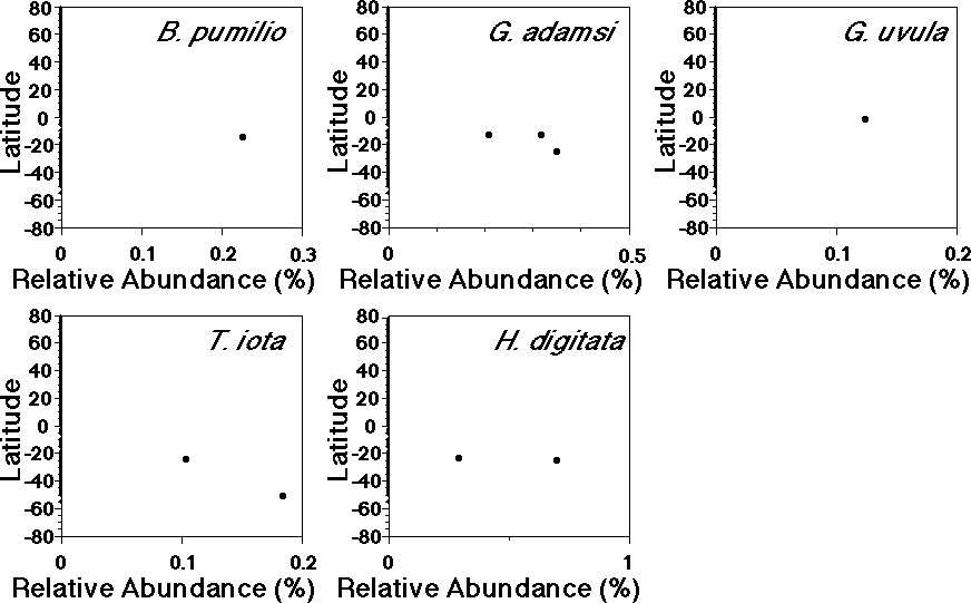
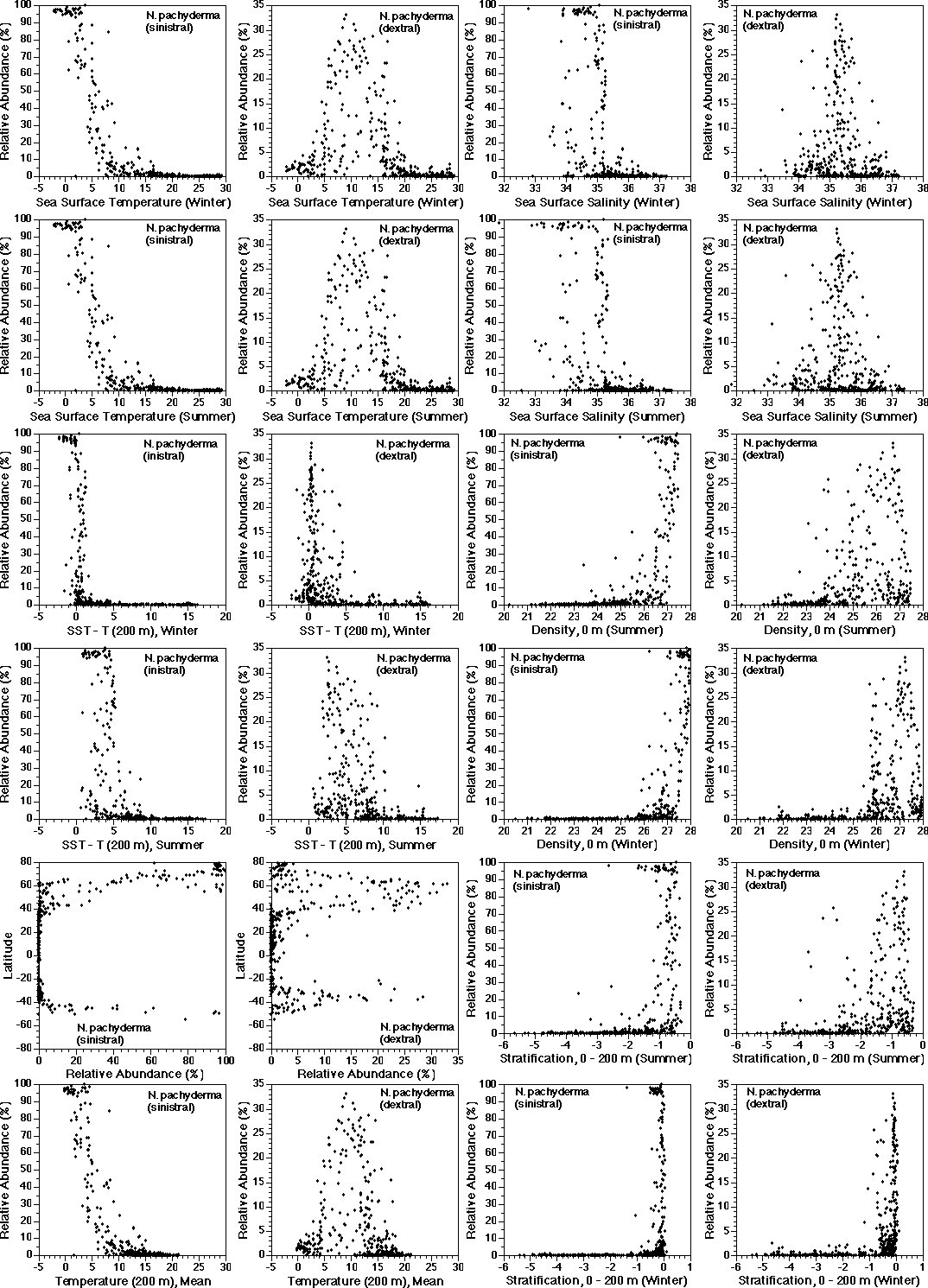
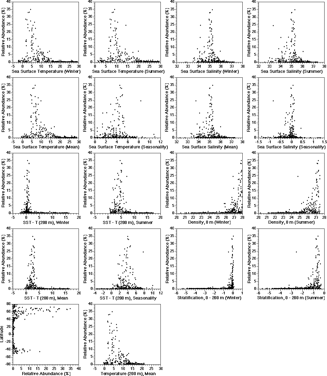
of your World Wide Web browser.


Fig. 1


Figure 1: Locations of 461 core top samples analysed by CLIMAP (1976, 1981), Béand Hutson (1977), and Kipp (1976) whose data is used in this paper. Geographic gaps in the data delineate areas of moderate to bad carbonate preservation from where samples have been excluded. Dark pattern marks shelf areas.


Fig. 2


Figure 2: Physical parameters extracted from the Levitus (1982) database and computed from this data. The depth of 200 m lies beyond most seasonal variation in the physical marine environment below the seasonal thermocline (Fig. 3). White lines indicate vertical temperature variation (schematic) in the major ocean areas. Note the different shape and strength of the seasonal thermocline and subsequent problems to define reprodicible levels, which would have made comparisons between different ocean areas and different seasons difficult.


Fig. 3


Figure 3: Correlation of summer and winter water temperatures at the sea surface and at 200 m depth based on oceanographic data extracted for each core location (Fig. 1) from the Levitus (1982) database. Note scatter in the correlation of sea surface temperatures and differences in the correlation between different segments of the data cloud. In the tropics a linear correlation hardly exists. Physical conditions at 200 m are nearly constant over the year and are used to characterise conditions below the seasonal thermocline.


Fig. 4


Figure 4: Plots of selected physical parameters (Fig. 2) vs. latitude for all sample locations used in this paper (Fig. 1). Data from Levitus (1982). See text for discussion.


Fig. 5


Figure 5: Relative abundances of species observed in only few samples plotted vs. latitude. See text for discussion.


Fig. 6


Figure 6: Candeina nitida d'Orbigny, 1839. Plots of relative abundance vs. selected physical parameters and latitude. For preferences in numeric form see appendix.


Fig. 7


Figure 7: Dentagloborotalia anfracta (Parker, 1967). Plots of relative abundance vs. selected physical parameters and latitude. For preferences in numeric form see appendix.


Fig. 8


Figure 8: Globigerina bulloides d'Orbigny, 1826. Plots of relative abundance vs. selected physical parameters and latitude. For preferences in numeric form see appendix.


Fig. 9


Figure 9: Globigerina falconensis Blow, 1959. Plots of relative abundance vs. selected physical parameters and latitude. For preferences in numeric form see appendix.


Fig. 10


Figure 10: Globigerinella digitata (Brady, 1879). Plots of relative abundance vs. selected physical parameters and latitude. For preferences in numeric form see appendix.


Fig. 11


Figure 11: Globigerinella calida (Parker, 1962). Plots of relative abundance vs. selected physical parameters and latitude. For preferences in numeric form see appendix.


Fig. 12


Figure 12: Globigerinella siphonifera (D'Orbigny, 1839) = G. aequilateralis (Brady). Plots of relative abundance vs. selected physical parameters and latitude. For preferences in numeric form see appendix.


Fig. 13


Figure 13: Globigerinita glutinata (Egger, 1895). Plots of relative abundance vs. selected physical parameters and latitude. For preferences in numeric form see appendix.


Fig. 14


Figure 14: Globigerinoides conglobatus (Brady, 1879). Plots of relative abundance vs. selected physical parameters and latitude. For preferences in numeric form see appendix.


Fig. 15a


Figure 15a: Globigerinoides ruber (D'Orbigny, 1839), differentiated for white and pink varieties. Plots of relative abundance vs. selected physical parameters and latitude. For preferences in numeric form see appendix. Continued in Fig. 15b and 15c.


Fig. 15b


Figure 15b: G. ruber continued. Plots of relative abundance vs. selected physical parameters and latitude. For preferences in numeric form see appendix. Continued in Fig. 15c.


Fig. 15c


Figure 15c: G. ruber continued.


Fig. 16


Figure 16: Globigerinoides sacculifer (Brady). Forms with sac chambers included. Plots of relative abundance vs. selected physical parameters and latitude. For preferences in numeric form see appendix.


Fig. 17


Figure 17: G. sacculifer with and without sac chamber: correlation of relative abundances, geographic distribution, and relation with water temperature at 200 m. For discussion see text.


Fig. 18


Figure 18: Globoquadrina conglomerata (Schwager, 1866). Plots of relative abundance vs. selected physical parameters and latitude. For preferences in numeric form see appendix.


Fig. 19


Figure 19: Globorotalia crassaformis (Galloway and Wissler, 1927). Plots of relative abundance vs. selected physical parameters and latitude. For preferences in numeric form see appendix.


Fig. 20


Figure 20: Globorotalia hirsuta (d'Orbigny, 1839). Plots of relative abundance vs. selected physical parameters and latitude. For preferences in numeric form see appendix.


Fig. 21


Figure 21: Globorotalia inflata (d'Orbigny, 1839). Plots of relative abundance vs. selected physical parameters and latitude. For preferences in numeric form see appendix.


Fig. 22


Figure 22: Globorotalia menardii (d'Orbigny, 1865). Plots of relative abundance vs. selected physical parameters and latitude. For preferences in numeric form see appendix.


Fig. 23


Figure 23: Globorotalia scitula Brady, 1882. Plots of relative abundance vs. selected physical parameters and latitude. For preferences in numeric form see appendix.


Fig. 24


Figure 24: Globorotalia truncatulinoides (d'Orbigny, 1839). Plots of relative abundance vs. selected physical parameters and latitude. For preferences in numeric form see appendix.


Fig. 25


Figure 25: Preferences for vertical temperature gradients and biogeographic distribution of Globorotalia truncatulinoides differentiated for sinistral and dextral coiling variants. For discussion see text.


Fig. 26


Figure 26: Globorotalia tumida (Brady, 1877). Plots of relative abundance vs. selected physical parameters and latitude. For preferences in numeric form see appendix.


Fig. 27


Figure 27: Correlation of relative abundances of Globorotalia tumida and G. tumida flexuosa; relations of G. tumida flexuosa with sea surface temperature in winter and summer, and its biogeographic distribution.


Fig. 28


Figure 28: Globorotaloides hexagonus (Natland, 1938). Plots of relative abundance vs. selected physical parameters and latitude. For preferences in numeric form see appendix.


Fig. 29


Figure 29: Globoturborotalita rubescens Hofker, 1959. Plots of relative abundance vs. selected physical parameters and latitude. For preferences in numeric form see appendix.


Fig. 30


Figure 30: Globoturborotalita tenella (Parker, 1958). Plots of relative abundance vs. selected physical parameters and latitude. For preferences in numeric form see appendix.


Fig. 31


Figure 31: Hastigerina pelagica (d'Orbigny, 1839). Plots of relative abundance vs. selected physical parameters and latitude. For preferences in numeric form see appendix.


Fig. 32


Figure 32: Neogloboquadrina dutertrei (d'Orbigny, 1839). Plots of relative abundance vs. selected physical parameters and latitude. For preferences in numeric form see appendix.


Fig. 33


Figure 33: Neogloboquadrina pachyderma (Ehrenberg, 1861). Plots of relative abundance vs. selected physical parameters and latitude. For preferences in numeric form see appendix.


Fig. 34


Figure 34: Neogloboquadrina pachyderma differentiated for sinistral and dextral coiling forms. Plots of relative abundance vs. selected physical parameters and latitude. For preferences in numeric form see appendix.


Fig. 35


Figure 35: Orbulina universa d'Orbigny, 1839. Plots of relative abundance vs. selected physical parameters and latitude. For preferences in numeric form see appendix.


Fig. 36


Figure 36: Pulleniatina obliquiloculata (Parker and Jones, 1865). Plots of relative abundance vs. selected physical parameters and latitude. For preferences in numeric form see appendix.


Fig. 37


Figure 37: Sphaeroidinella dehiscens (Parker and Jones, 1865). Plots of relative abundance vs. selected physical parameters and latitude. For preferences in numeric form see appendix.


Fig. 38


Figure 38: Turborotalita humilis (Brady, 1884). Plots of relative abundance vs. selected physical parameters and latitude. For preferences in numeric form see appendix.


Fig. 39


Figure 39: Turborotalita quinqueloba (Natland, 1938). Plots of relative abundance vs. selected physical parameters and latitude. For preferences in numeric form see appendix.


Fig. 40


Figure 40: G. bulloides and G. glutinata: biogeographic distributions (diameters of circles indicate relative abundances at a location), and correlation of relative abundances. The species co-occur in nearly all samples. See Figs. 8 and 13, and discussion section in the text.


Fig. 41


Figure 41: Range, suboptimum, and optimum as defined in this paper to extract information on preferences of species presented in the appendix.


Table


Table 1: Dominating species in at least one of the 461 samples analysed in this paper, ranked after mean relative abundance in the assemblages dominated by these species. Note that only the six most abundant species can be considered dominant on a biogeographic scale, and 6 species may dominate assemblages only in a few samples on a local scale. PD intergrades are forms intermediate between N. pachyderma and N. dutertrei.

Species
names

N. pachyderma
PD intergrade
G. inflata
G. bulloides
G. ruber
G. glutinata
G. menardii
T. quinqueloba
G. sacculifer
P. obliquiloculata
N. dutertrei
G. falconensis

Mean rel.
abundance

63.2
36.0
35.3
31.7
26.3
25.9
24.3
24.3
20.3
19.8
19.6
15.8

Standard
deviation

28.9
12.2
15.4
13.2
8.1
6.7
7.8
2.9
3.7
-
4.7
0.4

No. of
cases

104
3
47
49
191
21
25
2
6
1
4
6

Biogeographic
preferences

subpolar-polar
-
transitional
central cool productive
subtropical-marginal tropical
marginal cool productive
central tropical
-
-
-
-


back to table of contents